Optimizing Construction Schedules with Data Analytics

Understanding and Solving Construction Delays through Predictive Analytics
Construction delays are a persistent challenge plaguing the industry, leading to substantial financial losses and project inefficiencies. Grasping these delays’ nature, causes, and impact is crucial for developing effective mitigation strategies. Let’s delve deeper into the topic of construction delays and how predictive analytics can help solve this vexing issue.
The Grim Reality
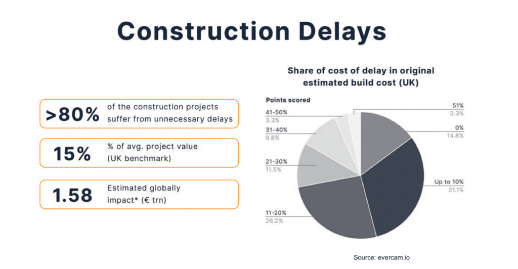
Studies have revealed that a staggering percentage of construction projects experience delays, with some estimates suggesting a sobering reality – up to 80% of projects are affected. The consequences are severe: cost overruns, reduced profitability, damaged reputations, and strained stakeholder relationships. The financial toll is particularly concerning, with reports indicating that the global construction industry loses billions of dollars annually due to delays.
- 80% of projects are delayed
- 31% of delayed projects are poorly managed
- Causing $1.7 trillion in losses due to project mismanagement
Common Culprits Behind Construction Delays
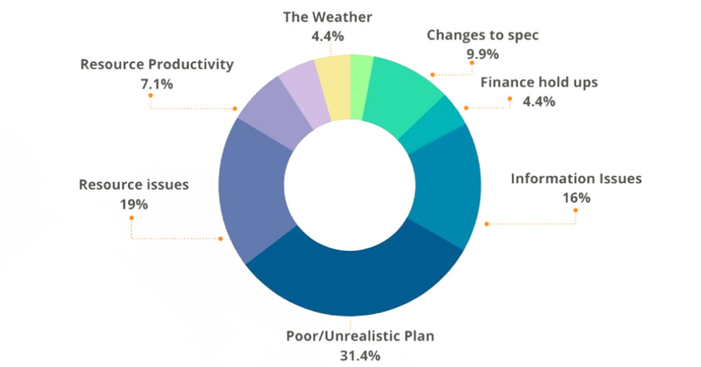
Delays in construction projects can stem from various factors. Poor project planning and scheduling, including inaccurate time and resource estimates, often set the stage for delays. Design changes and scope creep during construction disrupt carefully laid plans, throwing schedules into disarray. Inadequate resource allocation, such as insufficient labor or materials, hinders progress and causes bottlenecks. External factors like adverse weather conditions, heavy rain, or extreme temperatures can also impact activities negatively. Contractual and legal issues, including disputes or delays in obtaining permits, further contribute to project postponements. Finally, poor communication and coordination among team members and suppliers breed misunderstandings and rework, exacerbating delays.
The Role of Predictive Analytics: A Beacon of Hope
Predictive analytics emerges as a powerful tool to address construction delays effectively by improving project planning and resource management. By leveraging historical data, predictive models can provide more accurate time and resource estimates, reducing the likelihood of unrealistic scheduling from the outset. These models can also forecast potential design changes and scope creep, allowing for proactive adjustments to minimize disruptions. Moreover, predictive analysis optimizes resource allocation by identifying the most efficient distribution of labor, materials, and equipment, preventing shortages or surpluses that could impede progress. It can even predict adverse weather conditions, enabling better preparation and scheduling adjustments to mitigate their impact. Additionally, predictive tools can identify potential contractual and legal issues early, facilitating timely resolutions before they escalate into delays. Enhanced communication and coordination are achieved through predictive insights, which streamline workflows and reduce misunderstandings, ultimately minimizing delays caused by miscommunication or rework.
Predictive Analytics allows you to go beyond knowing what has happened and provide a best assessment of what will happen in the future.

The Fundamentals of Predictive Analytics
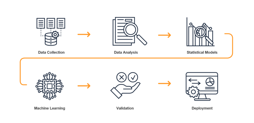
Predictive analytics harnesses historical data, statistical algorithms, and machine learning techniques to forecast future outcomes. It goes beyond merely understanding past events to provide insights into what might happen next. The process involves several key steps:
- Data Collection: Gathering relevant, high-quality data, such as project schedules, weather patterns, and resource allocation records.
- Data Analysis: Analyzing and cleaning the data to identify patterns and trends.
- Statistical Modeling: Applying statistical techniques like regression analysis to uncover hidden patterns and make predictions.
- Machine Learning: Utilizing algorithms like decision trees and neural networks to improve prediction accuracy over time.
- Validation: Testing the model’s performance on new data to ensure accuracy and reliability.
- Deployment: Integrating the validated model into existing systems to make real-time predictions and support data-driven decision-making.
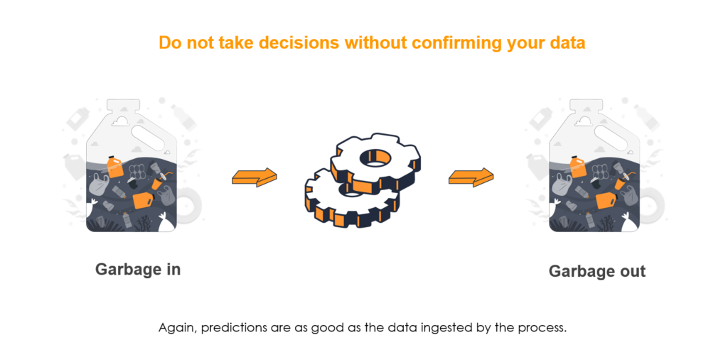
The Importance of Input Data Quality
It’s worth noting that the quality of predictions heavily depends on the quality of input data. The principle of “garbage in, garbage out” applies, meaning that the predictions will likely be unreliable if the input data is inaccurate, incomplete, or biased. Therefore, ensuring data quality and integrity is crucial for successful predictive analytics implementation.

Statistical Models: Decoding the Mathematical Representations
Statistical models are mathematical representations of real-world phenomena or relationships between variables. They are used to describe, explain, and predict the behavior of a system or process based on observed data. Commonly used machine learning models in construction scheduling include linear regression, decision trees, random forests, and neural networks.
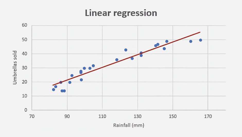
Linear regression predicts task duration or project timelines based on factors like resource allocation and task complexity by finding the best-fitting linear equation.
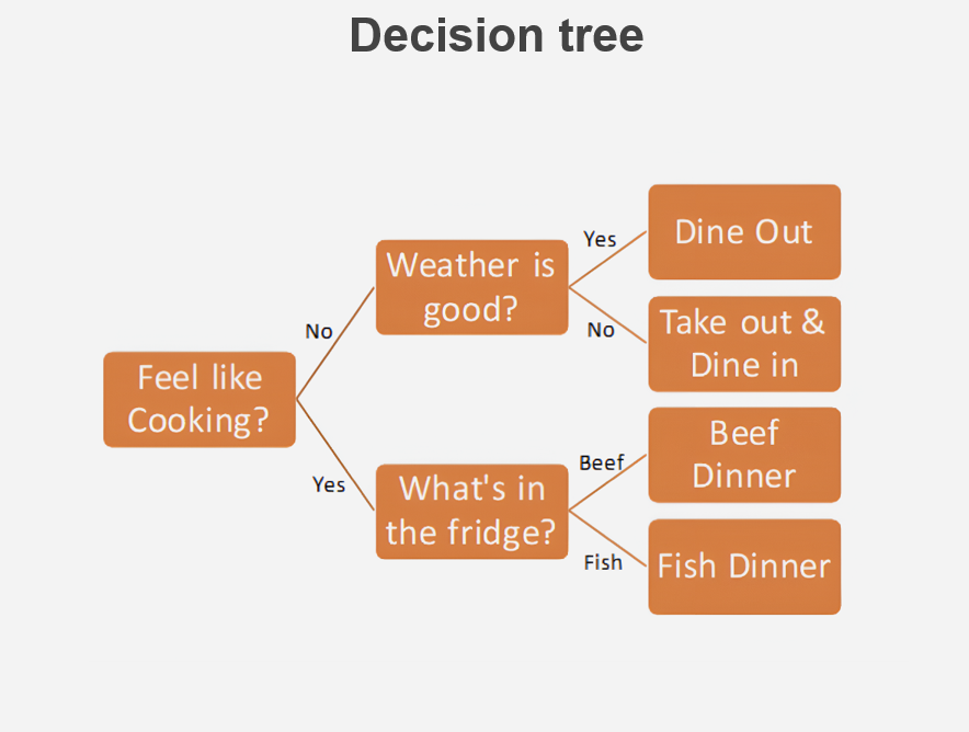
Decision trees predict delays by creating a tree-like structure based on factors such as project type and weather conditions.
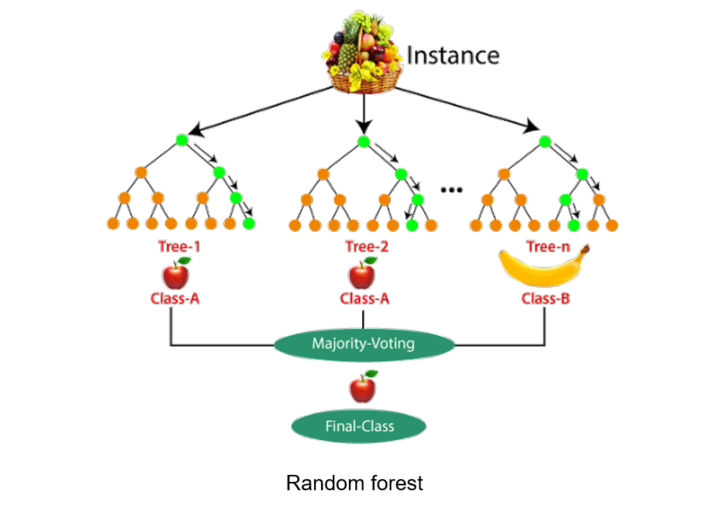
Random forests enhance decision trees by combining multiple trees trained on different data subsets, reducing overfitting and improving accuracy.
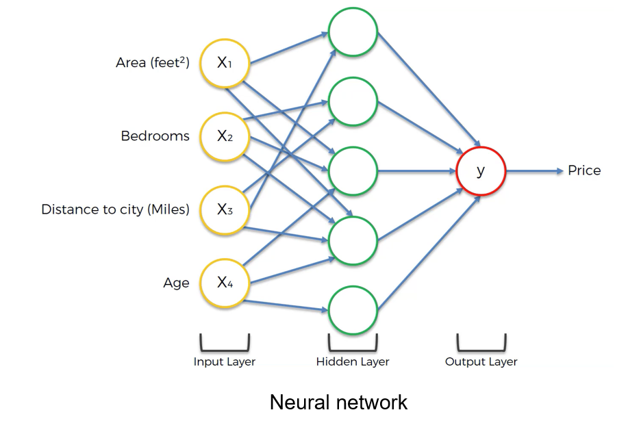
Inspired by the human brain, neural networks capture complex non-linear relationships, making them practical for learning intricate patterns in construction scheduling data.
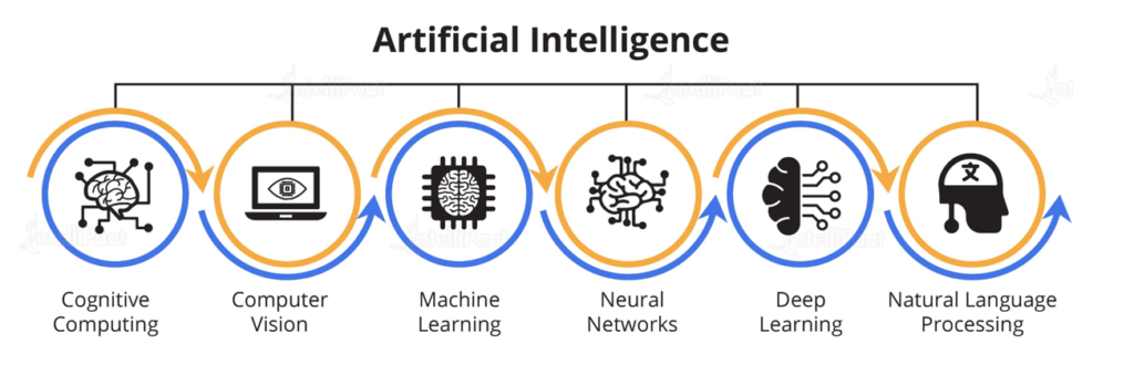
Demystifying Machine Learning
Machine learning is a field of study in artificial intelligence concerned with developing and studying statistical algorithms that can learn from data and generalize to unseen data, thus performing tasks without explicit instructions.
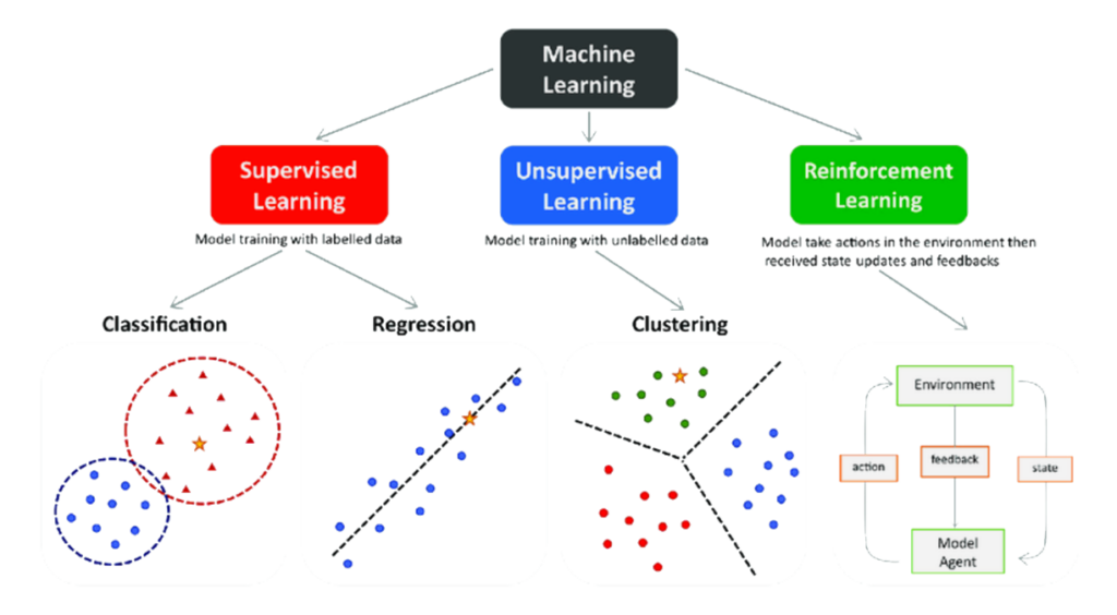
Categories of Machine Learning
Machine learning algorithms can be broadly categorized into three main types: supervised learning, unsupervised learning, and reinforcement learning. Each type serves different purposes and is suited for various tasks.
Supervised Learning:
- Regression Algorithms: Linear regression, polynomial regression, and support vector regression (SVR).
- Classification Algorithms: Logistic regression, decision trees, random forests, support vector machines (SVM), k-nearest neighbors (KNN), and neural networks.
Unsupervised Learning:
- Clustering Algorithms: K-means, hierarchical clustering, and DBSCAN (Density-Based Spatial Clustering of Applications with Noise).
- Dimensionality Reduction Algorithms: Principal component analysis (PCA), t-distributed stochastic neighbor embedding (t-SNE), and autoencoders.
- Association Algorithms: Apriori algorithm and Eclat algorithm.
Reinforcement Learning:
- Value-Based Algorithms: Q-learning and deep Q-networks (DQN).
- Policy-Based Algorithms: REINFORCE algorithm and proximal policy optimization (PPO).
- Model-Based Algorithms: AlphaGo and dynamic programming.
Additionally, hybrid algorithms combine elements from different types, such as semi-supervised learning and self-supervised learning, which leverage aspects of both supervised and unsupervised methods.
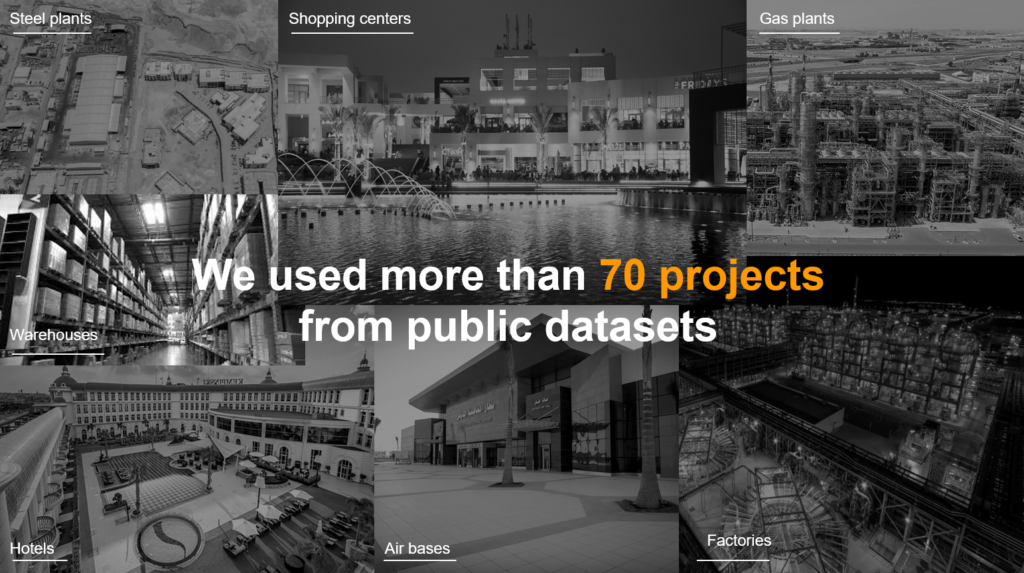
The Dataset: A Solid Foundation
To feed the machine learning algorithm, we needed a comprehensive dataset that was large enough and of good quality. As a basis, we required at least 50 construction projects with detailed Gantt charts estimated at the beginning of each project and the actual resulting Gantt chart after project completion. We found a dataset with more than 70 projects. After cleaning and normalizing the data, we uploaded all the projects to a repository for easy access (link provided in the original text).
The original dataset
The original dataset consisted of a list of Primavera files, which we exported and discarded any corrupt files, resulting in more than 300,000 data points.

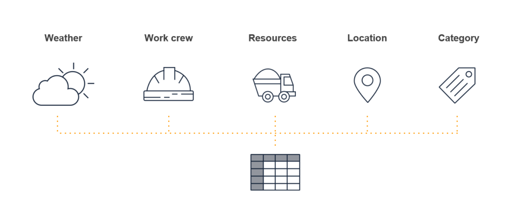
Impact Factors
We hypothesized that we would obtain certain factors that might affect task delays, such as category, location, resources, work crew, and weather. All of these factors were present in the dataset, except for weather. Given that all projects were built in the Egypt area between in 2010 and 2018, we obtained the average weather conditions for each month and used that as a baseline.
| Value Type | Jan | Feb | Mar | Apr | May | Jun | Jul | Aug | Sep | Oct | Nov | Dec |
| Precipitation Total (mm) | 4.77 | 3.75 | 6.28 | 1.34 | 0.21 | 0 | 0 | 0 | 0 | 0.73 | 4.29 | 3.4 |
| Days with Precipitation ≥ 1 mm | 1.3 | 2.03 | 1.17 | 1.3 | 0.6 | 0.57 | 0.67 | 1.03 | 0.73 | 0.13 | 0.63 | 0.83 |
| Daily Maximum Temperature (°C) | 18.93 | 20.53 | 23.81 | 28.11 | 32.19 | 34.62 | 35 | 34.93 | 33.36 | 29.98 | 24.93 | 20.52 |
| Daily Minimum Temperature (°C) | 10.08 | 10.99 | 13.16 | 15.92 | 19.31 | 22.2 | 23.79 | 24.27 | 22.72 | 19.95 | 15.6 | 11.7 |
| Daily Mean Temperature (°C) | 14.36 | 15.61 | 18.28 | 21.82 | 25.57 | 28.19 | 29.09 | 29.21 | 27.63 | 24.62 | 20.01 | 15.89 |
| Mean Sea Level Pressure (hPa) | 1019.1 | 1017.88 | 1015.79 | 1013.62 | 1012.35 | 1010.45 | 1008.19 | 1008.9 | 1012.14 | 1014.95 | 1017.05 | 1019.11 |
The Real Heroes: Data Processing Libraries
A high-quality dataset is critical for a project like this, but we also needed robust libraries to process the data effectively. For this exercise, we decided to use Python on Google Colab, primarily utilizing Scikit-Learn, Pandas, and NumPy as the main data processing libraries.

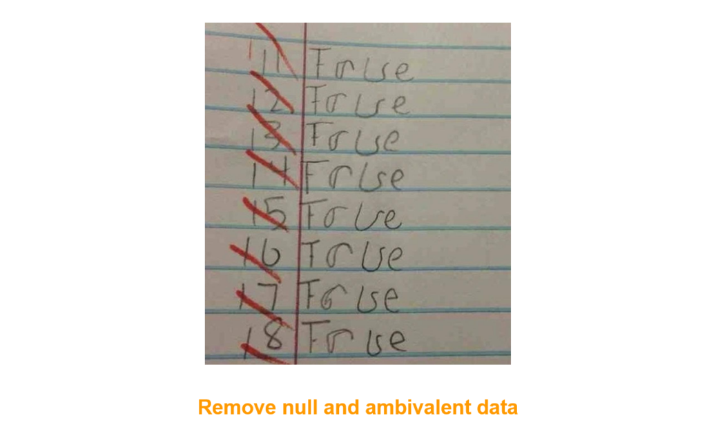
The Cleanup Process
The first part of the process was to remove all null data, outliers, or incomplete projects or milestones. We also cleaned tasks with uninformative names like codes or meaningless labels.
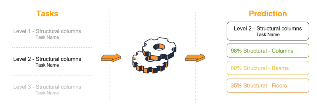
Defining Categories
We utilized machine learning to identify the categories of each column, ensuring standardization. For example, columns labeled “columns” and “pillars” were grouped into the “structural columns” category.
					# Load training data

df_train = pd.read_csv(training_data_path, usecols=['task_name', 'category', 'subcategory'])

# Prepare training and target datasets
X = df_train['task_name']
y = df_train[['category', 'subcategory']].astype(str).agg('_'.join, axis=1)

# Splitting the dataset for training and validation
X_train, X_test, y_train, y_test = train_test_split(X, y, test_size=0.2, random_state=42)

# Creating a text vectorization and classification pipeline
pipeline = make_pipeline(TfidfVectorizer(), SVC(kernel='linear', probability=True))

# Training the model
pipeline.fit(X_train, y_train)

# Validating the model
predictions = pipeline.predict(X_test)

# Save the model for later use
import joblib
joblib.dump(pipeline, 'category_predictor.joblib')
print(classification_report(y_test, predictions))
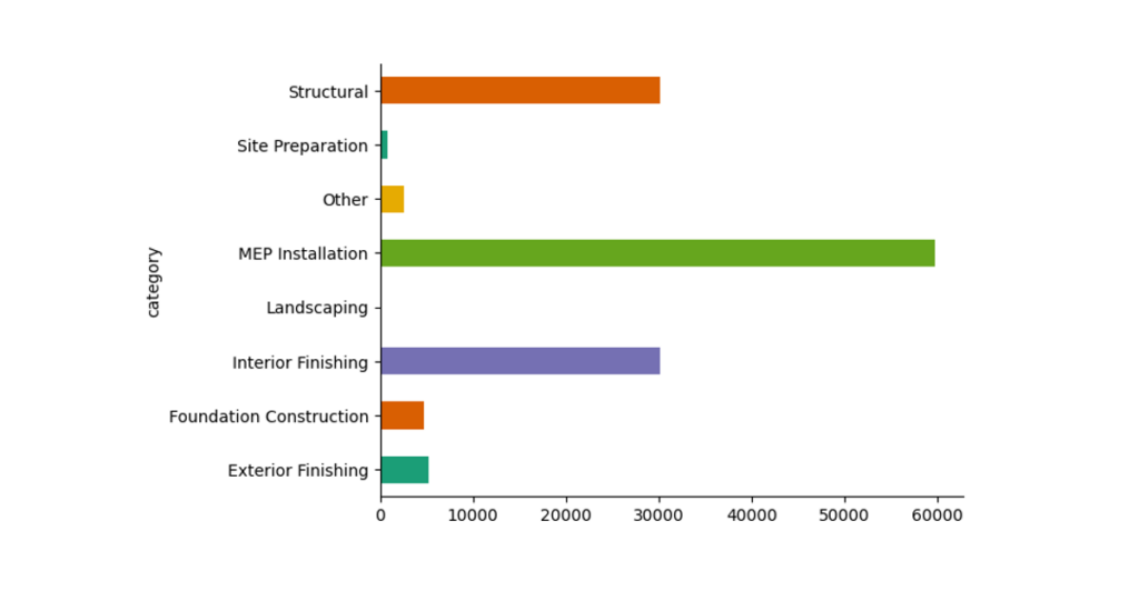
Elements grouped by category
We ended up with 8 categories. By far, the most crowded was MEP, followed by interior finishes and structural elements.
Transforming Variables into Numbers
The next step was transforming the variables into numerical values for the machine learning algorithm to understand. For example, Boolean values were converted to 0 or 1; Categories will be listed as 1, 2, 3, etc.
# reading the csv file classified_tasks.csv
# fill the missing values with 0
filtered_joined_df.fillna(
{col: 0 for col in filtered_joined_df.columns if filtered_joined_df[col].dtype != "object"}, inplace=True
)
# convert the date columns to datetime
date_columns = [x for x in filtered_joined_df.columns if "date" in x]
for col in date_columns:
filtered_joined_df[col] = pd.to_datetime(filtered_joined_df[col], errors="coerce")
# replace all N and Y with 1 and 0 respectively
filtered_joined_df.replace({"N": 0, "Y": 1}, inplace=True)
dates = [
["actual_d", "act_start_date", "act_end_date"],
["late_d", "late_start_date", "late_end_date"],
["early_d", "early_start_date", "early_end_date"],
["target_d", "target_start_date", "target_end_date"],
]
average_date = [
["actual_month", "act_start_date", "act_end_date"],
["late_month", "late_start_date", "late_end_date"],
["early_month", "early_start_date", "early_end_date"],
["target_month", "target_start_date", "target_end_date"],
]
columns = ["category", "subcategory","delay", "target_qty", "successors" ]
#fix missing dates columns, we will use
filtered_joined_df['act_start_date'] = filtered_joined_df['act_start_date'].fillna(filtered_joined_df['target_start_date'])
for date in average_date:
#get the average month between
filtered_joined_df[date[0]] = (filtered_joined_df[date[1]] + (filtered_joined_df[date[2]] - filtered_joined_df[date[1]])/2 ).dt.month
filtered_joined_df[date[0]] = filtered_joined_df[date[0]].astype("category").cat.codes
columns.append(date[0])
for date in dates:
#get the difference in days between the two dates
filtered_joined_df[date[0]] = (filtered_joined_df[date[1]] - filtered_joined_df[date[2]]).dt.days
columns.append(date[0])
filtered_joined_df["delay"] = filtered_joined_df["target_d"] - filtered_joined_df["actual_d"]
# replace strings with integers for columns category and subcategory
filtered_joined_df["category"] = filtered_joined_df["category"].astype("category").cat.codes
filtered_joined_df["subcategory"] = filtered_joined_df["subcategory"].astype("category").cat.codes
filtered_joined_df = filtered_joined_df[columns]
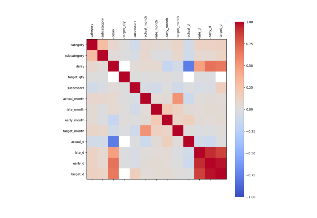
# draw correlation matrix with matplotlib
# use red color for negative correlation and blue color for positive correlation
# a value of 1 means perfect positive correlation
# a value of -1 means perfect negative correlation
# use column name as labels for the x and y axis
# x labeles to be vertical
# add range to graphical representation
plt.matshow(filtered_joined_df.corr(), cmap="coolwarm", vmin=-1, vmax=1)
plt.xticks(range(len(filtered_joined_df.columns)), filtered_joined_df.columns)
plt.xticks(rotation=90)
plt.yticks(range(len(filtered_joined_df.columns)), filtered_joined_df.columns)
plt.colorbar()
#make the plot bigger
plt.gcf().set_size_inches(10, 10)
# store it as a png file
plt.savefig("correlation.png")
filtered_joined_df.to_csv("processed.csv")
p = filtered_joined_df.corr()
p.to_csv("correlation.csv")
print(p)
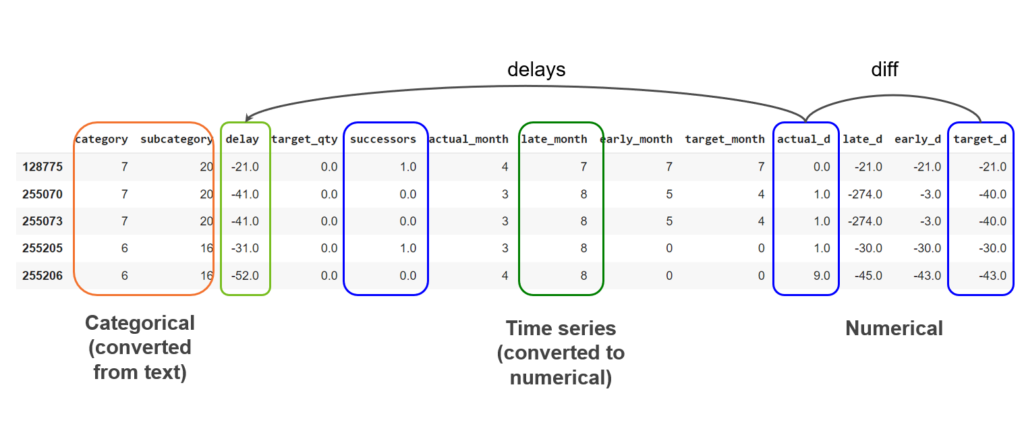
How the data looks
Below is a representation of how the data looks after the whole process, where Categorical information was converted into numbers and then the dates information.
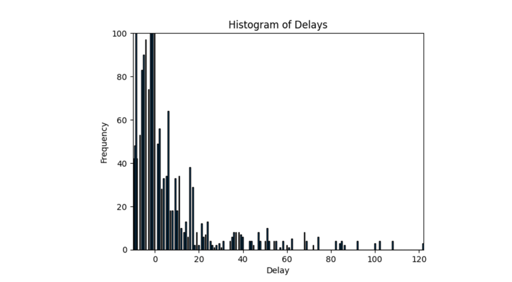
Task Delay Analysis
We created a graphic to illustrate how often tasks were completed in advance, on time, or delayed for each category. The good news is that many tasks were finalized in advance or on time. However, the problem was that many tasks experienced severe delays, which could have affected the entire construction process.
Correlation Analysis
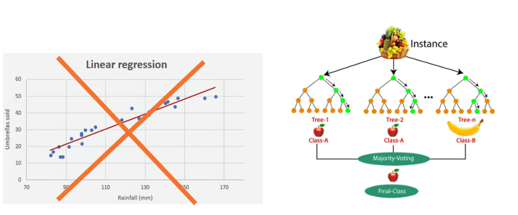
We conducted correlation analyses using Pandas to understand the data better. Notice that we needed to avoid the correlations between late, early, and target dates, given the complexity of the relationships. This meant we could not use linear regression, as the relationship was not strong enough. We needed to find a method that could categorize using factors with higher complexity.
The Selected Method: Random Forest – A Powerful Ensemble Approach
Based on the conclusions drawn from the correlation analysis, we decided to employ the random forest method, a powerful ensemble learning technique well-suited for handling complex relationships and high-dimensional data.
Random forest is an ensemble learning method used for classification, regression, and other tasks in machine learning. It operates by constructing a multitude of decision trees during the training phase and outputting the class that represents the mode of the classes (for classification problems) or the mean prediction (for regression problems) of the individual trees. The method combines the predictions from multiple trees to improve overall accuracy and control overfitting, resulting in a more robust and reliable model than a single decision tree.
Key features of random forests include:
- Bootstrap Aggregation (Bagging): Random forests leverage a technique called bagging, where each decision tree is trained on a random subset of the training data with replacement, meaning some samples may be repeated. This process helps reduce variance and improve the overall model’s stability.
- Random Feature Selection: At each split in the decision trees, a random subset of features is chosen from the total set of features, which helps create diverse trees and reduce correlation among them. This feature randomness further enhances the model’s ability to generalize and avoid overfitting.
- Ensemble Voting: For classification tasks, the final prediction is made by majority voting among the trees, where the class with the most “votes” is selected as the predicted class. For regression tasks, the prediction is the average of all the trees’ predictions, resulting in a more stable and accurate estimate.
- Handling Missing Data: Random forests can effectively handle missing values in the input data by incorporating them into the tree-building process, making them suitable for datasets with incomplete or partially missing information.
- Parallel Processing: Constructing individual trees in a random forest can be parallelized, allowing for efficient training on large datasets and faster model convergence.
This ensemble method helps handle large datasets with higher dimensionality. It can effectively deal with missing values, maintain accuracy even when a significant proportion of the data is missing, and capture complex non-linear relationships between features and the target variable.
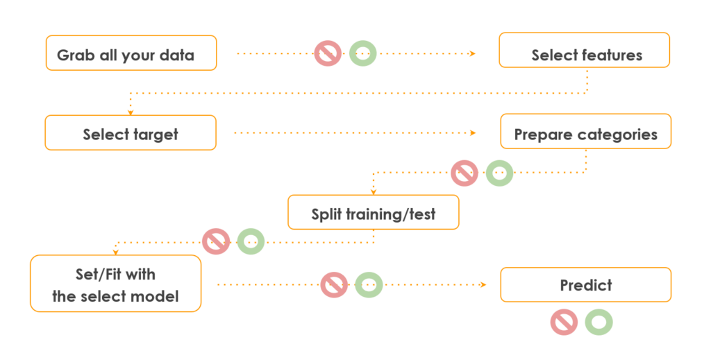
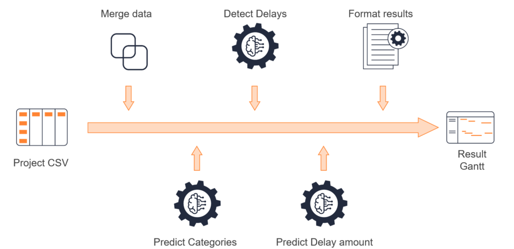
The whole process
As a recap this is how the process looks like from input data to prediction:
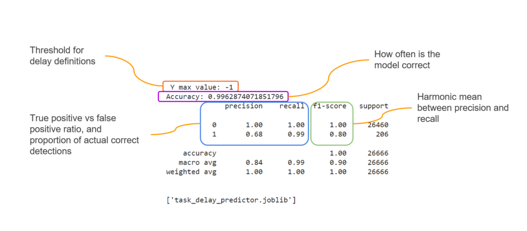
Model Performance Evaluation
To evaluate the performance of the trained model, we examine metrics such as precision and recall. Precision measures the proportion of optimistic predictions (delays) that are correctly identified, while recall measures the proportion of actual positive instances (true delays) that are correctly predicted by the model. Ideally, both precision and recall should tend towards 1, indicating high accuracy in detecting delays and correctly identifying non-delay instances. Additionally, we provide the average values of these metrics to give an overall sense of the model’s performance across different categories or scenarios.
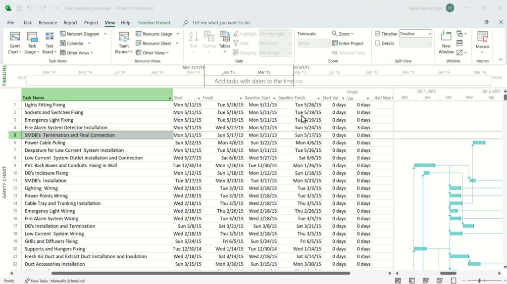
Using the Model for Predictions
To utilize the trained model for predictions, you can input a new project’s data (not used in the training set) as input. The model will then analyze the provided information and output the predicted delays, if any, along with their expected durations. It’s crucial to ensure that the input data is preprocessed and formatted consistently with the training data to obtain reliable predictions.
The result
In the video below, you can see an example of a result using our trained model.
Conclusions
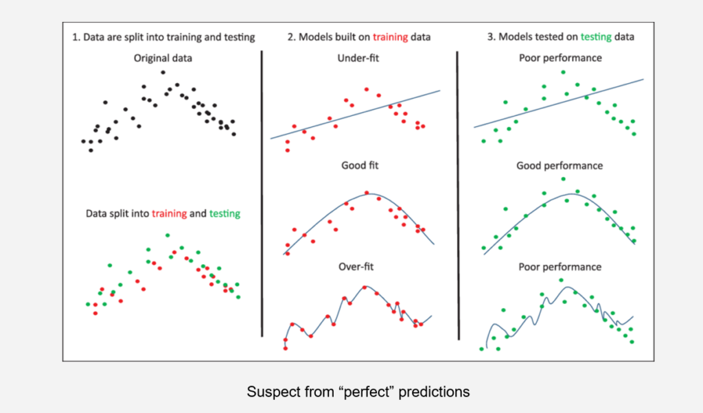
Check the quality of your data, if the datasets you are using are not complete, real or uncertain then the output of the model will not be good.
Check the quality of your data: If everything appears perfect, something might be amiss. Maintain a balance between underfitting and overfitting, performance, and training.
- Do not make decisions without confirming your data:
- Review projects to include only relevant data, as incomplete projects will add noise to the predictions.
- Create a category list that reflects your actual project structure.
- Use more than 30 projects to create a basic dataset, as a small dataset can return inaccurate values.
- If using projects from multiple locations, add locations as categorical data and include columns for average weather conditions.
We hope you found this post insightful and that it encourages you to train your own models and implement them for better forecasting of construction projects.
If you want to check the whole code, you can go to This repo.

Pablo Derendinger
https://www.e-verse.comI'm an Architect who decided to make his life easier by coding. Curious by nature, I approach challenges armed with lateral thinking and a few humble programming skills. Love to work with passioned people and push the boundaries of the industry. Bring me your problems/Impossible is possible, but it takes more time.